The Kaggle platform for analytical competitions and predictive modelling founded by Anthony Goldblum in 2010 is currently known almost to everyone who had contact with the area called Data Science. Thanks to its rich database, simplicity of operation and especially the community, it has become hugely popular over the years.

There are many manuals helping to open the door to the world of data exploration and modelling that encourages imagination. The majority of these manuals are based on the data including information on Titanic passengers, which is very accessible to understand.  Our goal is to determine the chances of surviving for each person as precisely as possible on the basis of their gender, age, travel class or place where their journey began. The examples use generally available tools and packages intended for modelling, i.e. R. Python or even Microsoft Excel, which is familiar to everyone. To my surprise, I did not manage to find even one complete example using one of the best tools for advanced analytics (SAS). There may be voices saying ‘SAS is not free of charge’ or ‘not everyone has access to SAS software’. Nothing could be more wrong! For a few years there already has been a free of charge, educational version of this software under the name of SAS University Edition. It contains all necessary components to start work with data and their modelling. The latest 3.6 version is extended with Jupyter Notebook which facilitates ordering codes, descriptions and analyses.

The purpose of the tutorial is to present how the functionalities of SAS University Edition can be used for teaching modelling. I do not want to discuss here the entire methodology of preparation for modelling, or data modelling as such. This field is so broad that the few articles would grow to the size of an entire book. The tutorial which I prepared became too long for a single entry; therefore, I had to divide it into several parts.

The first part of the tutorial will concern getting familiar with the data and basic analysis. Thanks to the insight into data, we will be able to draw initial conclusions and plan further steps.

In our next entry we will handle the logistic regression structure and assess its matching degree. We will also send the initial modelling results to Kaggle and wonder what we can do to improve the result awarded by Kaggle. The third part will consist in implementation of findings from the second entry. We will focus on engineering and extracting features, as well as check whether our additional work will bring any tangible results.

In these three entries we will rather focus on how to perform analyses in SAS UE and interpret results, but without going deeper into the SAS language syntax. If you are interested, please check two perfectly prepared free trainings in basics of SAS language and basics of data modelling in SAS. They provide solid foundations for working with this language.

• https://support.sas.com/edu/schedules.html?id=2588&ctry=PL
• https://support.sas.com/edu/schedules.html?id=2816&ctry=PL

The final part will not be a direct continuation of the tutorial, but it will be closely related to it. I will present a top shelf SAS tool intended for modelling, that is SAS Enterprise Miner, and we will use it for performing all previous analyses and modelling.  This will not be a training in the tool operation, but rather enumeration of advantages provided by this interface in comparison with writing codes as such.

The first step after installing and launching SAS University Edition will be to download data and import them in SAS. We will use for this the above-mentioned Titanic set, which can be found on Kaggle website. (https://www.kaggle.com/c/titanic/data). We download the train.csv file which will be used for modelling. The second file, test.csv, will be needed later. The sets should be uploaded to SAS Studio, the web-based interface of SAS programmer.

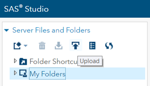
The uploaded data should be converted to the native SAS format. For this purpose, we will write the below code in the software window. We launch the entire software using F3 key, or its particular components by marking the lines which are interesting for us and pressing F3 key.

proc import file='/folders/myfolders/train.csv' out=train replace;run;

Two types of data can be distinguished in SAS: numeric and character. During the import, SAS automatically recognises and assigns the data types to the relevant variables.

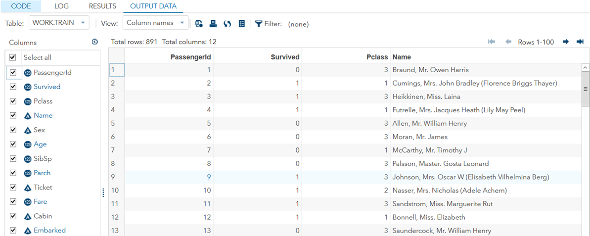
Before we begin modelling, we should get familiar with the data, i.e. determine the usefulness of variables, calculate the basic statistics, draw distribution, check the number of unique values and dependence with the dependent variable. The variable is Survived containing information whether the passenger survived (1) or not (0). The PassengerId variable is only a passenger identifier and will not be taken into consideration for modelling. Similarly in the case of Name and Ticket. Simple operations would allow us to obtain from these variables additional data which could prove to be useful. I will write about feature extraction some other time. The description of other variables is available on the Kaggle competition website and it is better to get familiar with it. Now we are moving to calculations at once.

title "Fundamental statistics for all numeric variables";proc means data=train nmiss mean std median min max;run;

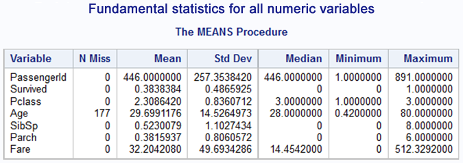
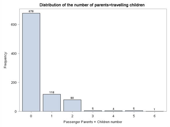
We will definitely have to face the missing data in the Age variable column. Pclass (travel class), SibSp (number of siblings + partner of travellers together) and Parch (number of children or parents travelling together) variables do not have this problem. On the other hand, judging by the description and scope of variables, it will be better to treat them as categorical variables. Let us see then what is the distribution of levels of these variables, as well as for the Survived variable and text variables.

title "Frequency tables for categorical variables in the training set";proc freq data=train nlevels;tables Survived;tables Sex;tables Pclass;tables SibSp;tables Parch;tables Embarked;tables Cabin;run;

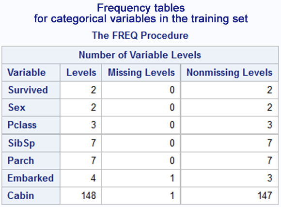
(part of results)

The number of Cabin variable levels is too high. In a standard case, we would have to reduce this number. Let us look at the table of frequencies.

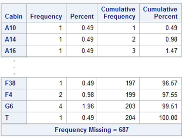
The number of missing values (687, i.e. approximately 77%) for this variable eliminates it from the list of variables for modelling. Additionally, will the passenger cabin number be a good predictor for whether someone will survive the disaster or not? Perhaps the letter before the number itself will introduce an additional value in modelling. We can take a closer look at this variable in the next approach to the problem solution. However, this time it will be skipped. We can see in the results what the proportions of particular variable levels are. Tables are not the easiest form of interpretation of values; therefore, let us use charts. The code for generating one of them has been placed below.

title "Distribution of embarkation locations";proc sgplot data=train;vbar Embarked / datalabel missing;label Embarked = "Passenger Embarking Port";run;

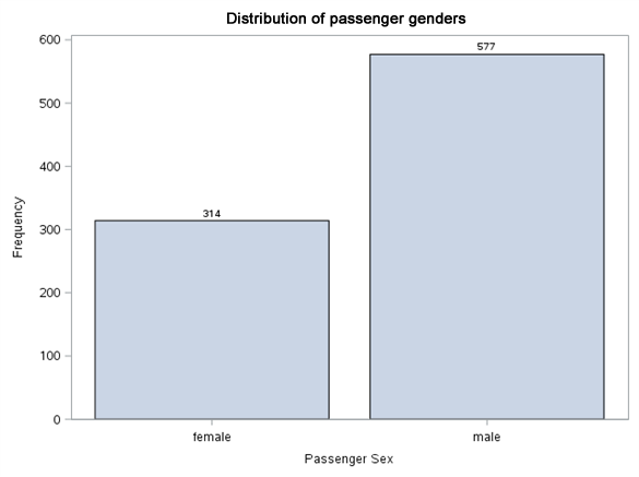
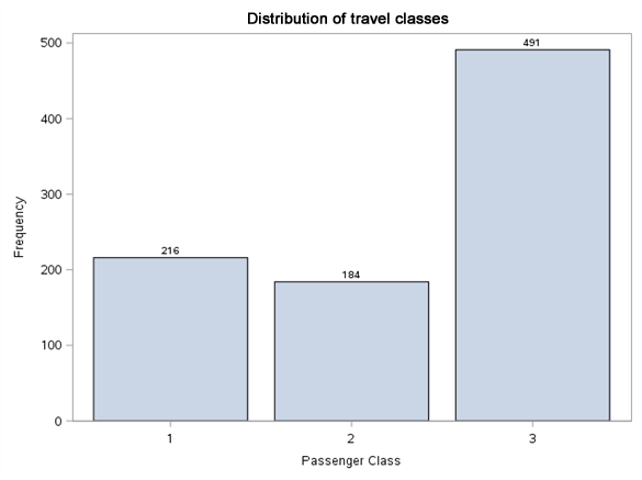
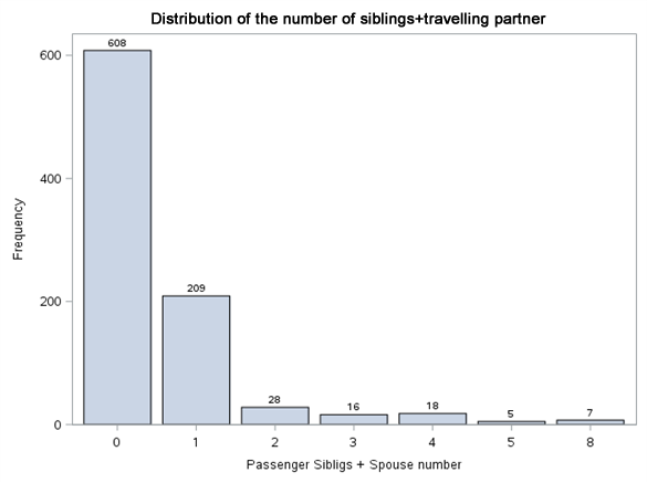
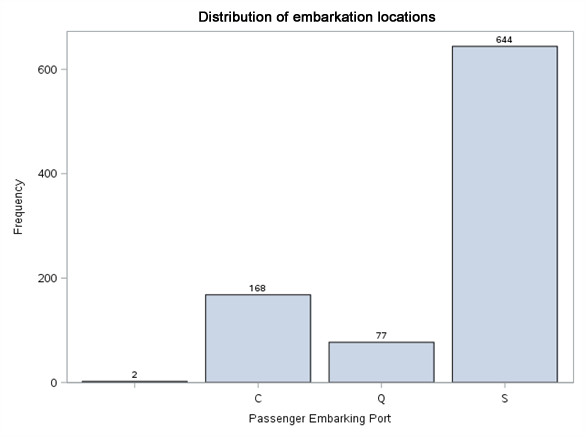
Nothing unusual can be seen in value distributions. We have two missing values in embarkation port. We will complete it with modal value (S). Let us see now what are the surviving proportions at particular levels of these variables.

title "Embarked vs Survived";proc sgplot data=train pctlevel=group;vbar Embarked / group=Survived stat=percent missing;label Embarked = "Passenger Embarking Port";run;

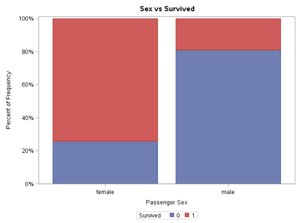
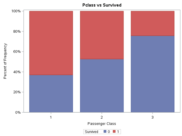
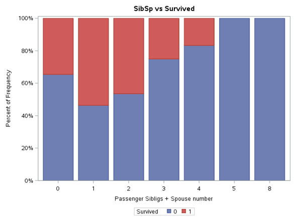
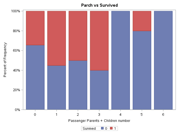
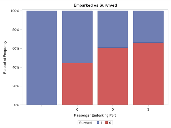
Each variable level was normalised to range 0%-100%. Thanks to such presentation of results, it is easier to notice the differences in proportion of Survived variable value between the levels of the same variable, as well as draw initial conclusions. Gender definitely has a very high impact on survivability. In line with the principle ‘women and children first’, it can be expected that the age will also play an important part in the model. The travel class also shows the tendency of higher survivability along with its growth. For SibSp variable, we may wonder whether values higher than 4 should be put into one bag. These levels are few in number and Survived variable adopts the value of 0 for them. A similar approach can be adopted for Parch variable.

Let us perform a similar analysis for constant variables.

title "Distribution of age value";proc sgplot data=train;histogram Age / binwidth=1;run;title "Age vs Survived";proc sgplot data=train;histogram Age / binwidth=1 group=Survived fillattrs=(transparency=0.5 );run;

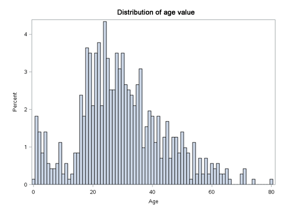
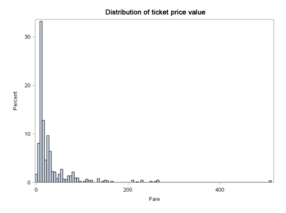
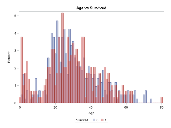
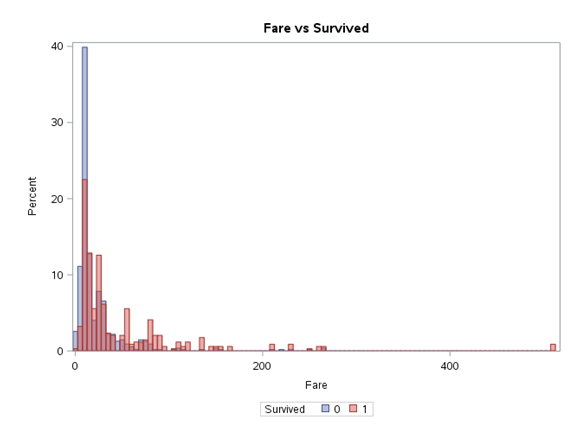
We may suppose that Fare variable is correlated with Pclass variable. A higher travel class means a higher ticket price. We can either reject one of them, or allow the modelling algorithm to decide which one will be better. With the Age variable it can be seen that the survival rate in the group aged up to 15 (children) is higher. Then it decreases, while at the end it slightly increases again. This increase at the end can also be related to the socioeconomic status.

After performing such initial analysis we already know what data we can expect, and we are also able to plan further steps that will prepare them for modelling. In the next entry, we will handle the completion of missing data and develop a simple model to be tested by means of data from test.csv file.