Kaggle with SAS - part two
- 4 September 2017
- Posted by: Piotr Florczyk
- Category: Publications

In the previous part of the cycle entitled ‘Kaggle with SAS – first steps with data’, we explored data by means of SAS University Edition (hereinafter referred to as SAS UE) to get familiar with their basic characteristics. This time we will handle the initial data preparation and develop a simple classification model using logistic regression.
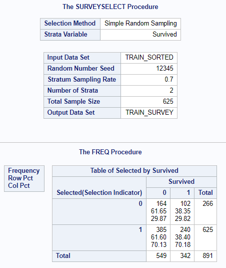
Before we begin modelling, we should divide data into two parts, i.e. training and validation. This is a typical procedure used in order to avoid the so-called ‘model overtraining’ and facilitate its quality assessment. In case of developing multiple models, the validation set may be used for selection of the best of them. The usually applied division patterns are 50/50 (50% for training part and 50% for validation part), 60/40, 70/30 or 80/20. This depends on the modeller’s preferences and amount of data at our disposal. The division cannot be accidental. We must be confident that both parts have equal proportions of the variable that we will model; therefore, stratified sampling shall be applied. For this purpose, we will use the surveyselect procedure available at SAS UE. The procedure requires a data set to be sorted by the stratifying variable. In order to verify the correct data division, it is worth generating a frequency table.
proc sort data=train out=train_sorted; by Survived;run;proc surveyselect data=train_sorted out=train_survey outall samprate=0.7 seed=12345; strata Survived;run;proc freq data=train_survey; tables Selected*Survived;run;

The Selected variable with the value of 1 will mean observation of the training part. Let us also perform quick set processing in order to leave only the columns that are interesting for us and name variables properly.
data titanic; set train_survey; rename Selected=Part; drop SelectionProb SamplingWeight;run;
Logistic regression is perfect for modelling binary variable (such as the Survived variable). In order to develop and use a model, we must be confident that each observation has a complete set of data, i.e. all columns for particular observation have assigned values. Let us remind how many data are missing in particular variables (data from the previous article of our cycle):
| Variable | Number of missing data |
| Age | 177 (19.87%) |
| Embarked | 2 (0.22%) |
| Fare | 0 (0.00%) |
| Parch | 0 (0.00%) |
| Pclass | 0 (0.00%) |
| Sex | 0 (0.00%) |
| SibSp | 0 (0.00%) |
The Age variable has as many as 177 cases of missing data. This constitutes almost 20% of the set. If we began modelling based on uncompleted data, the algorithm would reject these 20% of observations. Thus, we would lose a very large amount of information included in the set. We updated the missing data among the classification variables in Embarked variables. In the previous article we decided to skip the Cabin variable and not to use it in modelling due to excessive number of levels and huge proportion of missing data (approximately 77%). We will return to it in the following part of the article.
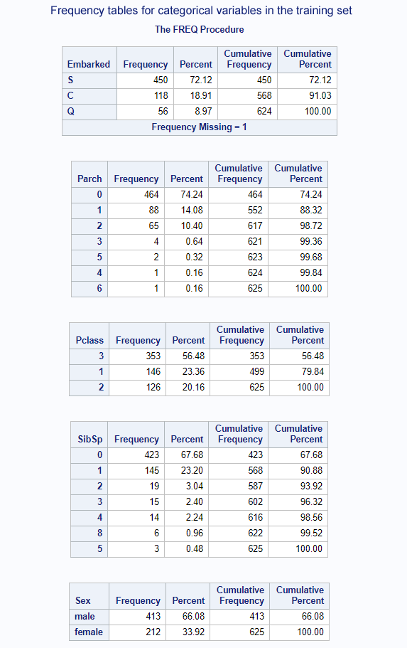
We will replace missing data for constant variables with the average values, and for the categorical variables with the medians. The imputed values should be calculated based on the training part, and then used to complete both the training and validation parts. Although there are no missing data in certain variables, it is worth protecting ourselves against such possibility. Therefore, the code will be prepared so as to also take such variables into consideration.
title "Average for Age and Fare variables in the training set";proc means data=titanic mean; where part=1; var Age Fare;run;
title "Frequency tables for categorical variables in the training set";proc freq data=titanic order=freq; where part=1; tables Embarked; tables Parch; tables Pclass; tables SibSp; tables Sex;run;
The above codes will indicate us the values for imputation of missing data.


Let’s perform the imputation, then.
data titanic; set titanic; if Age = . then Age = 29.63; if Embarked = ' ' then Embarked = 'S'; if Fare = . then Fare = 32.05; if Parch = . then Parch = 0; if Pclass = . then Pclass = 3; if Sex = ' ' then Sex = 'male'; if SibSp = . then SibSp = 0;run;
Now we can begin modelling. For this purpose, we will use the logistic procedure on training data. The generated model will be recorded, and then used for scoring of all observations. Then we will check in how many cases our model was wrong or right by means of division into training and validation data.
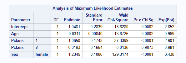
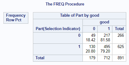
proc logistic data=titanic; where part=1; class Embarked Parch Pclass Sex SibSp Survived; model Survived(event='1') = Age Fare Embarked Parch Pclass Sex SibSp / selection=stepwise expb; store titanic_logistic;run;proc plm source=titanic_logistic; score data=titanic out=titanic_scored predicted=p / ilink;run;data titanic_model_score; set titanic_scored; if Survived = 1 and p > 0.5 then good = 1; else if Survived = 0 and p <= 0.5 then good = 1; else good = 0;run;proc freq data=titanic_model_score; tables part*good / nocol nopercent;run;

The variable selection algorithm decided that the model will include Age, Pclass and Sex variables.

The proportion of correctly classified cases (good=1) is approximate both for the training set (Part=1) and validation set (Part=0). It amounts to 79.20% and 81.58% for the training and validation sets respectively. Thanks to this, we can see that we obtained a stable model with a decent result without high work expenditure.
Let’s see how we perform in a competition. In order to send our result, we need to perform scoring of test.csv data set and send the result to Kaggle website.
proc import file="/folders/myfolders/test.csv" out=test replace;run;
data test; set test; if Age = . then Age = 29.63; if Embarked = ' ' then Embarked = 'S'; if Fare = . then Fare = 32.05; if Parch = . then Parch = 0; if Pclass = . then Pclass = 3; if Sex = ' ' then Sex = 'male'; if SibSp = . then SibSp = 0;run;proc plm source=titanic_logistic; score data=test out=test_scored predicted=p / ilink;run;data test_scored; set test_scored; if p > 0.5 then Survived = 1; else Survived = 0; keep PassengerId Survived;run;proc export data=test_scored file="/folders/myfolders/simple_logistic.csv" replace;run;

Taking into consideration the fact that we use only three variables for the model, the result of 75.12% is not bad. We still have a few columns at our disposal, so we can afford more. Our goal is minimum 80%. What can we do to improve this result?
- In names we can find the title of a particular person, i.e. Mr, Mrs, Miss, Don, Sir, etc.
- It may look stupid, but let’s try to calculate the name length.
- Ticket numbers repeat in subsequent observations. There are probably family and single tickets.
- Let’s search for the Titanic plans online. Perhaps we can indicate on the basis of cabin numbers where a particular cabin was located. Deck, left/right board, stern, etc.
As we can see, there are still many ideas worth verifying, because it may turn out that we will be able to obtain much more information from the data than we had initially assumed. All this will come in the following part.

AUTHOR
Piotr Florczyk
Graduate of the Electronic and Information Science Department at Warsaw University of Technology in the field of Electronics, Information Technology and Telecommunications. He worked for over five years at SAS Institute Polska where he developed his coaching skills, as well as gained knowledge and experience by participating in projects. He was a trainer, coach and presented at multiple conferences organised by SAS. He specialises in business analytics and processing large volumes of data in dispersed systems.
